Forward vs Reverse KL Divergence: Why the Direction Matters

If you've ever trained a variational autoencoder, fine-tuned a language model, or implemented policy optimization in reinforcement learning, you've encountered KL divergence. But here's the catch: there are two ways to compute it, and they lead to fundamentally different behaviors.

Most machine learning practitioners know that KL divergence measures how different two probability distributions are. What's less obvious is that $D_{KL}(P||Q) \neq D_{KL}(Q||P)$. This asymmetry determines whether your model will be conservative or risky, whether it covers all modes or focuses on one, and ultimately shapes how your training behaves.

While this topic has been discussed before, most explanations stay abstract. This post takes a different approach: we'll implement a toy example from scratch, visualize the actual optimization dynamics, and then systematically connect the behavior to diverse ML applications from language model pretraining to RLHF, VAEs, and knowledge distillation. By the end, you'll have both the intuition and the practical context to recognize which KL divergence you're using and why it matters.

A Quick Reminder: What is KL Divergence?

In simple terms, KL divergence measures how one probability distribution differs from another:

Or in the continuous case:

It's always non-negative, and equals zero only when P and Q are identical. (Can you see why? Hint: Jensen's Inequality.) Jensen's inequality states that for a convex function f: E[f(X)] ≥ f(E[X]). Apply this to -log (which is convex) and the ratio P(x)/Q(x).

Ok so KL feels like some kind of distance measure... or is it? How can it be a distance measure when it's not symmetric!

In reality, KL measures how inefficient it is to pretend samples come from $Q$ when they really came from $P$. Think about it as some sort of a penalty. If you know the true distribution $P$, you get zero KL. Negative KL would mean you did better than the true distribution P, but since you can't do better on average → no negative KL.

So to unwrap this asymmetry, we will do a simple experiment. But before that, let's give more context to the problem. Talking about probability distributions P and Q in abstract terms might be confusing, so let's connect it to something we already know.

In the context of LLM training, think of it this way:

• P: the target distribution: could be your data distribution (your corpus), the reference model, or a teacher model
• Q: your model: the one you're actively training and updating, usually an LLM, policy/student/etc.

For example:

• In pretraining language models, P is the true data distribution and Q is your LLM learning to approximate it
• In RLHF, P is your pre-trained base model (to prevent drift) and Q is your policy being optimized with RL (both LLMs in this case)
• In knowledge distillation, P is the teacher model and Q is the student

With this convention:

• Forward KL: $D_{KL}(P||Q) = \mathbb{E}_{x \sim P}\left[\log \frac{P(x)}{Q(x)}\right]$ becomes expectation under the target P
• Reverse KL: $D_{KL}(Q||P) = \mathbb{E}_{x \sim Q}\left[\log \frac{Q(x)}{P(x)}\right]$ becomes expectation under your model Q

The Experiment: Fitting a Unimodal to a Bimodal Distribution

Ok so what's the big deal? What happens when you choose one over the other? What do we usually use in practice?

To answer all these questions, we'll do a simple toy experiment. Consider the following scenario:

• Target P: A bimodal Gaussian mixture with two equally weighted Gaussians centered at x = -2 and x = +6, each with unit variance
• Model Q: A single Gaussian with parameters $\mu$ (mean) and $\sigma$ (standard deviation) that we'll optimize

This setup mirrors real ML problems: your data (or reference/teacher model) has multiple modes, but your model has limited capacity. How does the choice of KL divergence affect what Q learns?

Setting Up the Distributions

First, let's define an abstract class for a probability distribution. We want it to have two methods:

• sample: Since we have expectations, we will need to do Monte Carlo estimation, i.e., to generate and average over random samples from the distribution Exact KL is rarely computed in modern ML systems. Expectations are intractable, so KL is usually estimated from samples, so we'll do that as well.
• log_prob: This method computes the log-probability of a given input under the distribution, simply to compute the $\log P(x)$ and $\log Q(x)$ that appear in the equations above.

class Distribution(ABC):
    """
    Abstract base class for probability distributions.
    All distributions must implement sample() and log_prob().
    """
    
    @abstractmethod
    def sample(self, n_samples):
        """Draw n_samples from the distribution."""
        pass
    
    @abstractmethod
    def log_prob(self, x):
        """Compute log probability density at x."""
        pass

Next, if you forgot your probabilities (shame on you), let's remind ourselves what a simple 1-D Gaussian Distribution looks like

where $\mu$ is the mean and $\sigma$ is the standard deviation. Now let's implement the two methods:

sample: We could naively sample using a built-in function such as torch.normal(mean=self.mu, std=self.sigma, size=(1, n_samples)). This produces correct samples but it causes a problem once we start training.

Remember that when optimizing our model Q(x), we are actually learning the parameters μ and σ. With direct sampling, the randomness is injected inside the sampling operation itself, which makes the output non-differentiable with respect to these parameters. As a result, gradients cannot properly flow back to μ and σ.

To restore differentiability, we use the reparameterization trick: This trick was popularized by Kingma & Welling in their 2014 VAE paper, enabling backpropagation through stochastic nodes.

Now the source of randomness is entirely isolated in ε, which is independent of the learnable parameters. The sampling step becomes a deterministic function of μ and σ, allowing gradients to flow cleanly through the computation graph.

log_prob: Starting from the Gaussian density:

class GaussianDistribution(Distribution):
    """Gaussian Distribution for gradient-based optimization."""
    
    def __init__(self, mu, sigma):
        self.mu = torch.as_tensor(mu, dtype=torch.float32).requires_grad_(True)
        self.sigma = torch.as_tensor(sigma, dtype=torch.float32).requires_grad_(True)
    
    def sample(self, n_samples):
        """Reparameterization trick: x = mu + sigma * eps"""
        eps = torch.randn(n_samples)
        return self.mu + self.sigma * eps
    
    def log_prob(self, x):
        """Compute log P(x) for torch tensors."""
        return -0.5 * torch.log(2 * torch.pi * self.sigma**2) - 0.5 * (x - self.mu)**2 / self.sigma**2

Now let's define our target distribution P(x), a mixture of Gaussians. A Gaussian Mixture Model (GMM) with K components can be written as

• $\pi_k$ are the mixture weights
• $\mu_k$ are the component means
• $\sigma_k$ are the component standard deviations

sample: Drawing from a mixture follows the definition directly:

1. Sample a discrete component index $z \sim \mathrm{Categorical}(\pi_1,\ldots,\pi_K)$
2. Sample from the chosen Gaussian component $x \sim \mathcal{N}(\mu_z, \sigma_z^2)$

In this experiment, $P(x)$ is a fixed reference distribution: we are not optimizing its parameters, so we don't need the sampling operation to be differentiable. That means we can use simple numpy sampling (fast and straightforward) without worrying about the reparameterization trick.

log_prob: Computing $\log P(x)$ requires care. Recall that for a mixture:

so we need to find a numerically stable log-sum-exp formulation. Let's derive it below:

This expression is exactly a log-sum-exp. Computing it naively can be numerically unstable when some $a_k(x)$ values are very large or very small. Without the max subtraction, exp(a_k) can overflow to infinity or underflow to zero, causing NaN gradients. This trick is standard in softmax implementations too.

To stabilize the computation, we use the standard identity:

where $m = \max_k a_k$. This is what the code below implements.

class GaussianMixtureDistribution(Distribution):
    def __init__(self, means, sigmas, weights):
        self.means = torch.tensor(means, dtype=torch.float32)
        self.sigmas = torch.tensor(sigmas, dtype=torch.float32)
        self.weights = torch.tensor(weights, dtype=torch.float32)
        self.weights = self.weights / self.weights.sum()  # normalize
        self.n_components = len(means)
    
    def sample(self, n_samples):
        """Sample from the mixture"""
        components = np.random.choice(
            self.n_components, 
            size=n_samples, 
            p=self.weights.numpy()
        )
        samples = np.random.normal(
            self.means.numpy()[components],
            self.sigmas.numpy()[components]
        )
        return torch.tensor(samples, dtype=torch.float32)
    
    def log_prob(self, x):
        """Compute log P(x) using log-sum-exp trick"""
        log_probs = []
        for i in range(self.n_components):
            log_gaussian = -0.5 * torch.log(2 * torch.pi * self.sigmas[i]**2) \
                          - 0.5 * (x - self.means[i])**2 / self.sigmas[i]**2
            log_probs.append(torch.log(self.weights[i]) + log_gaussian)
        
        log_probs = torch.stack(log_probs)
        max_log = torch.max(log_probs, dim=0)[0]
        return max_log + torch.log(torch.sum(torch.exp(log_probs - max_log), dim=0))

Computing KL

Next, let's see how to compute the KL divergence in practice. Forward KL is defined as:

The key detail is the distribution inside the expectation: samples are drawn from $P$.

In practice, we approximate this expectation using Monte Carlo:

1. Sample $x^{(i)} \sim P(x)$
2. Evaluate $\log P(x^{(i)})$ and $\log Q(x^{(i)})$
3. Average the difference

We already have our handy functions, which makes the code very simple:

def forward_kl(p, q, n_samples=10000):
    """
    Compute KL(P||Q) = E_P[log P(x) - log Q(x)]
    Sample from P, evaluate both P and Q.
    """
    x = p.sample(n_samples)
    return torch.mean(p.log_prob(x) - q.log_prob(x))

Reverse KL swaps the roles:

Now the expectation is taken under Q, i.e. we sample from the model itself.

def reverse_kl(p, q, n_samples=10000):
    """
    Compute KL(Q||P) = E_Q[log Q(x) - log P(x)]
    Sample from Q, evaluate both Q and P.
    """
    x = q.sample(n_samples)
    return torch.mean(q.log_prob(x) - p.log_prob(x))

Forward KL: Minimizing KL(P||Q)

Finally! Let's get to the optimization part we've been waiting for. To keep things simple, we will not use a built-in PyTorch optimizer. Instead, we will implement simple gradient descent. But we don't have to worry about computing the gradient ourselves. We can leave that part to PyTorch's autograd.

By the way, if you're thinking to yourself: “Wait… I've fine-tuned models before and I never explicitly used a KL loss?” You're not wrong. Since $\log P(x)$ is constant, doesn't depend on $Q$'s parameters, we can safely drop it and minimizing $-\mathbb{E}_{x \sim P}[\log Q(x)]$ is equivalent, and that's just the familiar cross-entropy (negative log-likelihood) loss you're probably used to in PyTorch! This is why you'll rarely see "forward KL" mentioned explicitly in pretraining code.

def optimize_forward_kl(p, mu_init=0.0, sigma_init=1.0, lr=0.1, n_steps=1000, n_samples=1000):
    """
    Optimize Q to minimize KL(P||Q) using gradient descent.
    
    Loss: E_P[-log Q(x)]
    Sample from P (fixed), compute -log Q(x), backprop through Q's parameters.
    """
    # Initialize Q's parameters
    mu = torch.tensor(mu_init, requires_grad=True)
    sigma = torch.tensor(sigma_init, requires_grad=True)
    
    loss_history = []
    
    for step in range(n_steps):
        # Create Q with current parameters
        q = GaussianDistribution(mu, sigma)
        
        # Compute loss: E_P[-log Q(x)]
        loss = forward_kl(p, q, n_samples)
        
        # Backprop
        loss.backward()
        
        # Gradient descent update
        with torch.no_grad():
            mu -= lr * mu.grad
            sigma -= lr * sigma.grad
            
            # Zero gradients
            mu.grad.zero_()
            sigma.grad.zero_()
        
        loss_history.append(loss.item())
        
        if step % 100 == 0:
            print(f"Step {step}: Loss = {loss.item():.4f}, mu = {mu.item():.4f}, sigma = {sigma.item():.4f}")
    
    return mu.item(), sigma.item(), loss_history

Output:

Step 0: Loss = 8.8810, mu = 0.1893, sigma = 2.9083
Step 100: Loss = 0.7901, mu = 1.1521, sigma = 4.0272
Step 200: Loss = 0.7516, mu = 1.5349, sigma = 4.1245
Step 300: Loss = 0.7012, mu = 1.7554, sigma = 4.1338
Step 400: Loss = 0.7414, mu = 1.8741, sigma = 4.1251
Step 500: Loss = 0.7162, mu = 1.9375, sigma = 4.1203
Step 600: Loss = 0.7091, mu = 1.9555, sigma = 4.1231
Step 700: Loss = 0.7588, mu = 1.9747, sigma = 4.1216
Step 800: Loss = 0.7579, mu = 1.9890, sigma = 4.1182
Step 900: Loss = 0.7465, mu = 1.9980, sigma = 4.1202
Final parameters: mu = 1.9926, sigma = 4.1189

Let's visualize!

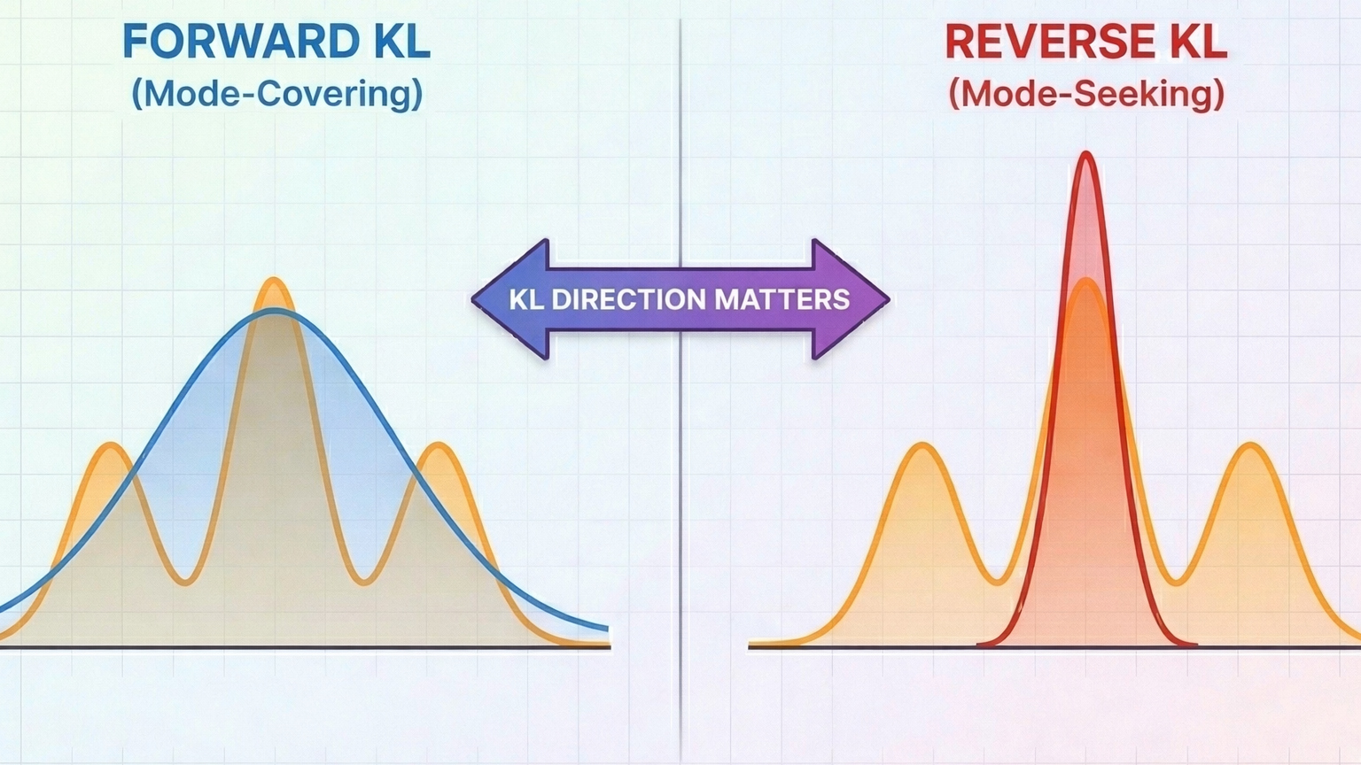
What happened? Recall our target P has modes at x = -2 and x = +6. Q learned to center itself at μ ≈ 2 (between the two modes) with a large σ ≈ 4.1 that covers both peaks.

Why? We're sampling from P and maximizing $\log Q(x)$, meaning we are asking $Q$ to explain the samples from $P$. So when x comes from either mode of $P$, $Q$ must assign reasonable probability to both regions. If $Q$ focused on just one mode, it would assign near-zero probability to samples from the other, leading to $\log Q(x) \rightarrow -\infty$.

This is mode-covering behavior: forward KL penalizes Q heavily when Q(x) ≈ 0 but P(x) > 0.

Reverse KL: Minimizing KL(Q||P)

Now let's check out what happens in the other direction.

def optimize_reverse_kl(p, mu_init=0.0, sigma_init=1.0, lr=0.01, n_steps=1000, n_samples=1000):
    """
    Optimize Q to minimize KL(Q||P) using gradient descent.
    
    Loss: E_Q[log Q(x) - log P(x)]
    Sample from Q using reparameterization, compute log Q(x) - log P(x), backprop.
    """
    # Initialize Q's parameters
    mu = torch.tensor(mu_init, requires_grad=True)
    sigma = torch.tensor(sigma_init, requires_grad=True)
    
    loss_history = []
    
    for step in range(n_steps):
        # Create Q with current parameters
        q = GaussianDistribution(mu, sigma)
        
        # Compute loss: E_Q[log Q(x) - log P(x)]
        loss = reverse_kl(p, q, n_samples)
        
        # Backprop
        loss.backward()
        
        # Gradient descent update
        with torch.no_grad():
            mu -= lr * mu.grad
            sigma -= lr * sigma.grad
            
            # Zero gradients
            mu.grad.zero_()
            sigma.grad.zero_()
        
        loss_history.append(loss.item())
        
        if step % 100 == 0:
            print(f"Step {step}: Loss = {loss.item():.4f}, mu = {mu.item():.4f}, sigma = {sigma.item():.4f}")
    
    return mu.item(), sigma.item(), loss_history

Output:

Step 0: Loss = 2.6755, mu = -0.0181, sigma = 1.0046
Step 100: Loss = 0.9817, mu = -1.2403, sigma = 1.0532
Step 200: Loss = 0.7341, mu = -1.7184, sigma = 1.0109
Step 300: Loss = 0.6986, mu = -1.9010, sigma = 1.0004
Step 400: Loss = 0.6933, mu = -1.9620, sigma = 0.9978
Step 500: Loss = 0.6935, mu = -1.9849, sigma = 0.9978
Step 600: Loss = 0.6932, mu = -1.9952, sigma = 0.9995
Step 700: Loss = 0.6930, mu = -2.0038, sigma = 1.0004
Step 800: Loss = 0.6928, mu = -2.0021, sigma = 0.9946
Step 900: Loss = 0.6931, mu = -2.0001, sigma = 1.0030
Final parameters: mu = -2.0000, sigma = 1.0037

Completely different! Q collapsed onto the left mode: $\mu ≈ -2$, $\sigma ≈ 1$. It ignored the right mode entirely.We initialized μ = 0 (closer to the left mode) to break symmetry. Starting at $\mu = 2$ could converge to either mode. This initialization sensitivity is a real issue in practice. Reverse KL can get stuck in local optima, which is why techniques like annealing or multiple restarts are sometimes used.

Why? We are sampling from $Q$ and evaluating $\log P(x)$. In other words, we use $P$ to score samples proposed by $Q$. Any mass that $Q$ places in low-probability regions of $P$ (e.g. between the modes, where $P(x) \approx 0$) gets heavily penalized since $\log P(x) \to -\infty$.

The safest strategy is therefore to concentrate all probability mass in a single high-density region of $P$. To assign non-negligible mass to both modes, a unimodal Gaussian must widen, which inevitably increases mass in low-density regions (including between the modes). Reverse KL penalizes that. The result: pick one mode and commit. Nothing to lose.

This is mode-seeking behavior: reverse KL penalizes Q when Q(x) > 0 but P(x) ≈ 0.

The Takeaway

Here's the intuition to remember:

• Forward KL $D_{KL}(P||Q)$: "Encourages behavioral cloning, prioritizes coverage" You sample from the target P and ask Q to explain those samples. If P has probability somewhere and Q doesn't, you get infinite penalty. Result: Q spreads out to cover all of P's modes, even if it means putting mass in low-probability regions Mode-covering, conservative, recall-oriented.
• Reverse KL $D_{KL}(Q||P)$: "Encourages specialization, prioritizes precision" You sample from your model Q and ask P to validate those samples. If Q puts mass where P doesn't, you get infinite penalty. Result: Q collapses onto P's highest-density regions and ignores the rest. Mode-seeking, confident, precision-oriented.

More Examples

There are many more interesting examples: variational autoencoders, knowledge distillation, and out-of-distribution detection. Sometimes both forward and reverse KL may be viable depending on the data and desired outcome.

I want to share a nice real-world example in a paper I recently read where the direction of KL matters. The paper is trying to solve machine unlearning. Wang et al. “Balancing Forget Quality and Model Utility: A Reverse KL-Divergence Knowledge Distillation Approach for Better Unlearning in LLMs.” NAACL 2025. Paper Suppose a language model was trained on data containing a sensitive fact, such as "John Smith's SSN is 123-45-6789." The goal is to remove this specific fact while keeping the rest of the model intact and useful.

The authors define a small forget set containing the data to be erased, and construct a teacher distribution that explicitly downweights tokens whose probabilities were boosted by this forget set (for example, the SSN digits), while leaving unrelated behavior unchanged. But the teacher model is not great, it has a deliberately distorted distribution meant only to guide learning.

They then distill a student model from this teacher using reverse KL. Because reverse KL weights errors by the student's own probabilities, it strongly penalizes the model whenever it assigns high probability to forbidden tokens. If the student still tries to output “123-45-6789,” reverse KL “hammers” it. Forward KL, by contrast, would be more forgiving and could allow some leakage.

Estimating KL in Practice

A final note: When reading ML papers and code, you might be surprised to see KL written in a completely different form. For example, in the famous DeepSeek R1 paper, they use this formula: Guo et al. "DeepSeek-R1: Incentivizing Reasoning Capability in LLMs via Reinforcement Learning." arXiv 2025. Paper

While this might seem weird, remember that in practice we always estimate KL using Monte Carlo sampling because computing the exact expectation is intractable. The textbook discrete KL formula then becomes just one of many possible Monte Carlo estimators, and a naive one at that!

This goes back to the age-old question of estimators: the bias-variance trade-off. The naive Monte Carlo estimator $\frac{1}{N}\sum_i \log \frac{P(x_i)}{Q(x_i)}$ can have high variance. A single sample where $Q(x)$ is very small (but $P(x)$ is not) can dominate the entire estimate and cause extreme variance.

For that reason, people look for better estimators. I won't expand more here as this has been extensively discussed. A good resource is John Schulman's blog post where he tests different KL estimators. His conclusion? A particularly effective low-variance estimator adds a correction term to the naive estimator: Schulman, J. "Approximating KL Divergence." Blog post a great deep dive into practical KL estimation.

Look familiar? That's exactly what the DeepSeek paper uses :)

Hamad, Hassan, "Forward vs Reverse KL Divergence: Why the Direction Matters", hassanhamad.com, Jan 2026.

@article{hamad2026kl,
  author = {Hassan Hamad},
  title = {Forward vs Reverse KL Divergence: Why the Direction Matters},
  journal = {hassanhamad.com},
  year = {2026},
  note = {https://hassanhamad.com/blog/forward-vs-reverse-kl/},
}